
The Metamorphosis
From Pairs to Portfolio
Part 4 of 6: Statistical Arbitrage for Independent Traders
Previously:
A Tale of Two Prices (the core idea of stat arb)
Moneyball (finding good pairs using metrics that matter)
The Winter of our Pairs Trading Discontent (problems, limitations, frustrations)
Pairs trading remains a feasible approach for the indie trader. But, as we saw last time, there are inherent limitations. Trading both legs eats a lot of buying power and limits the number of pairs you can trade.
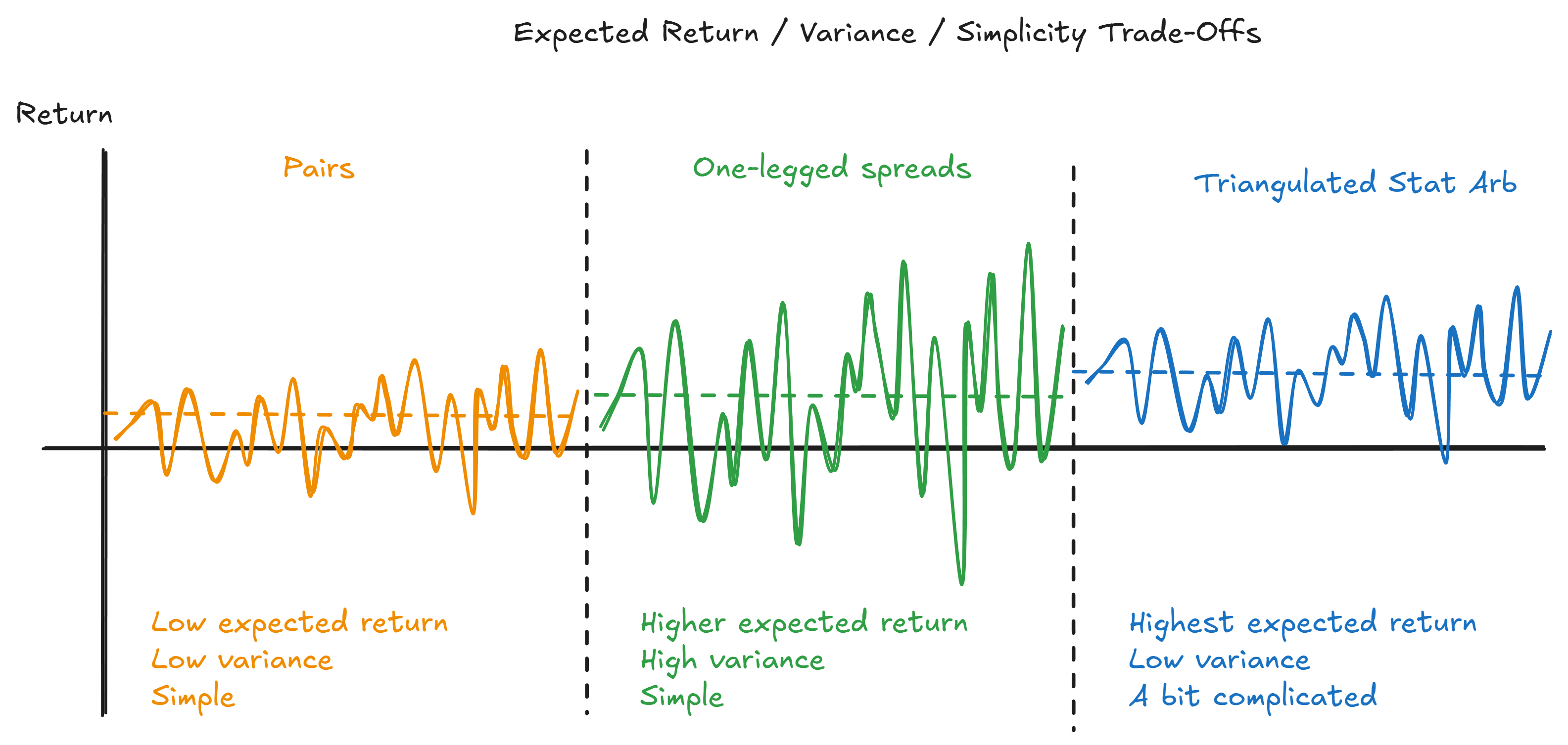
Trading only the mispriced leg helps, but introduces a ton of variance. Essentially, the trade-off is accepting a wilder ride in exchange for higher expected returns and better capital efficiency.
In the last article, I alluded to an approach that might offer a third route: we give up a little simplicity, but in exchange, we get higher expected returns and some variance control.
Here’s an example based on a small universe of spreads constructed from energy stocks. Six stocks, eight spreads.
Here are the z-scores of these spreads:
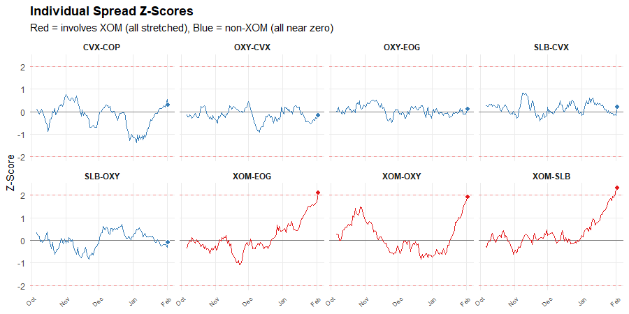
Every spread involving XOM is stretched. The spreads not involving XOM are all near zero. SLB, CVX, OXY, EOG, COP trade fairly against each other. XOM is the outlier.
The network of overlapping spreads tells us something specific: XOM is the mispriced security.
In Part 3, we talked about the constraints of traditional pairs trading. You trade spreads because it gives you built-in variance reduction. Long one leg, short the other, and you’re insulated from broad market moves. That’s valuable.
But you pay for it. Half your capital sits on a leg that might be fairly priced. You pay double the transaction costs. And when your selection pipeline identifies 100 good pairs but you can only trade 10, most of your signal goes unused.
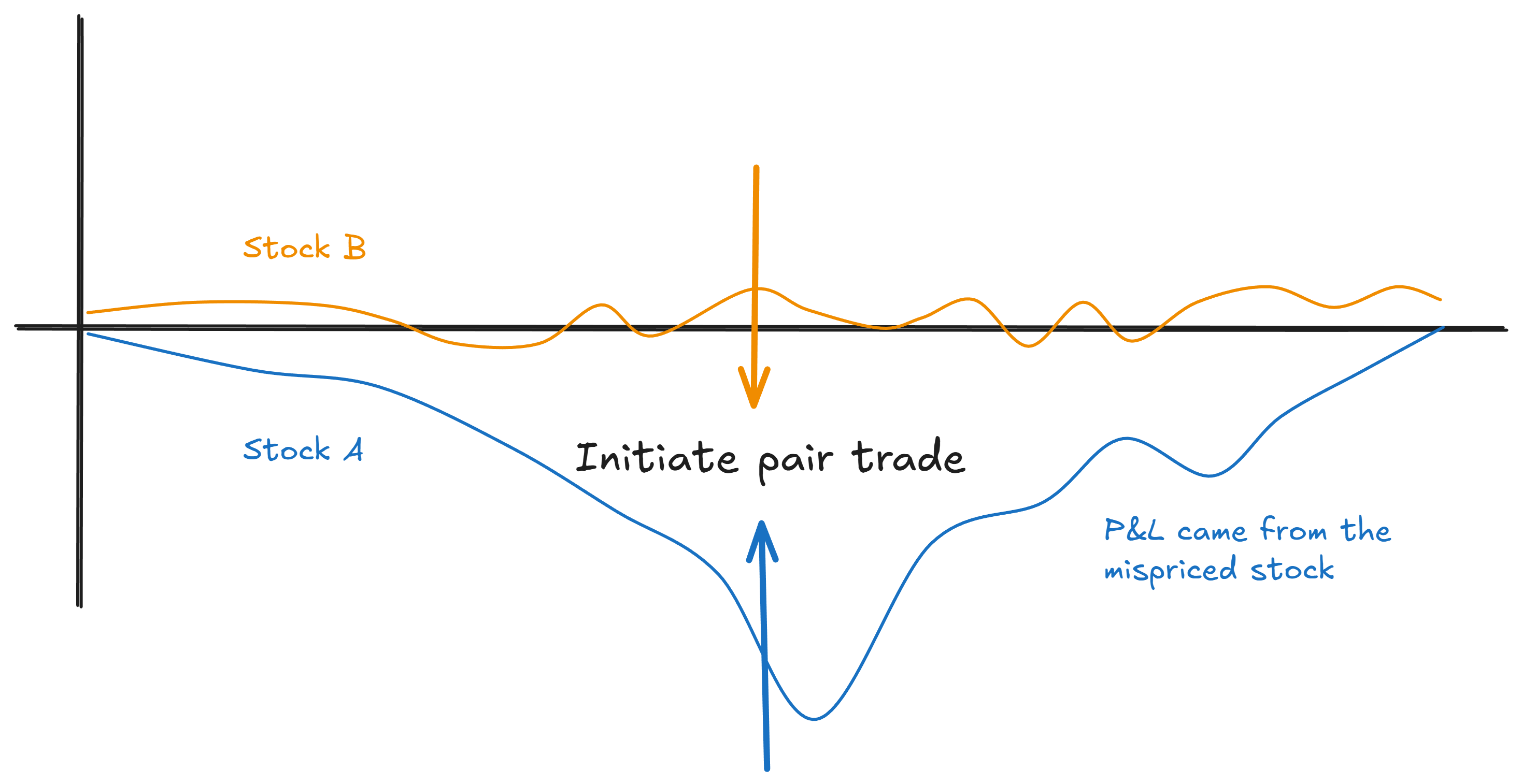
Now, you could try to trade just the mispriced leg. With a handful of pairs, you might even identify it by observing which stock moved. If XOM rallied 10% while SLB was flat, XOM probably drove the divergence.
But that’s not foolproof. Sometimes stocks move on beta, and the one left behind is actually the mispriced leg. “Which one moved” is useful information, but it’s not the whole picture.
One thing you can do is directly model market- and even sector-beta in your spread construction.
That’s a useful thing to do on average. If you can build a better model, then you should, all else being equal.
But that’s a big “if.”
Betas aren’t stable, and they’re prone to measurement error:
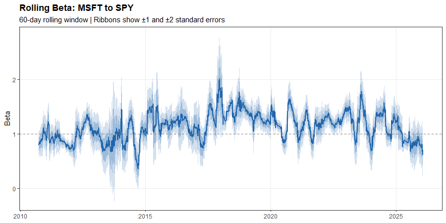
It’s difficult to model this stuff well in a way that’s of practical benefit to the trader.
But there’s another source of information here that’s hiding in plain sight, requires little modelling skill to extract, and is relevant right at the time you measure it.
I’m referring to the network of interconnected tickers that arises from a collection of overlapping spreads:
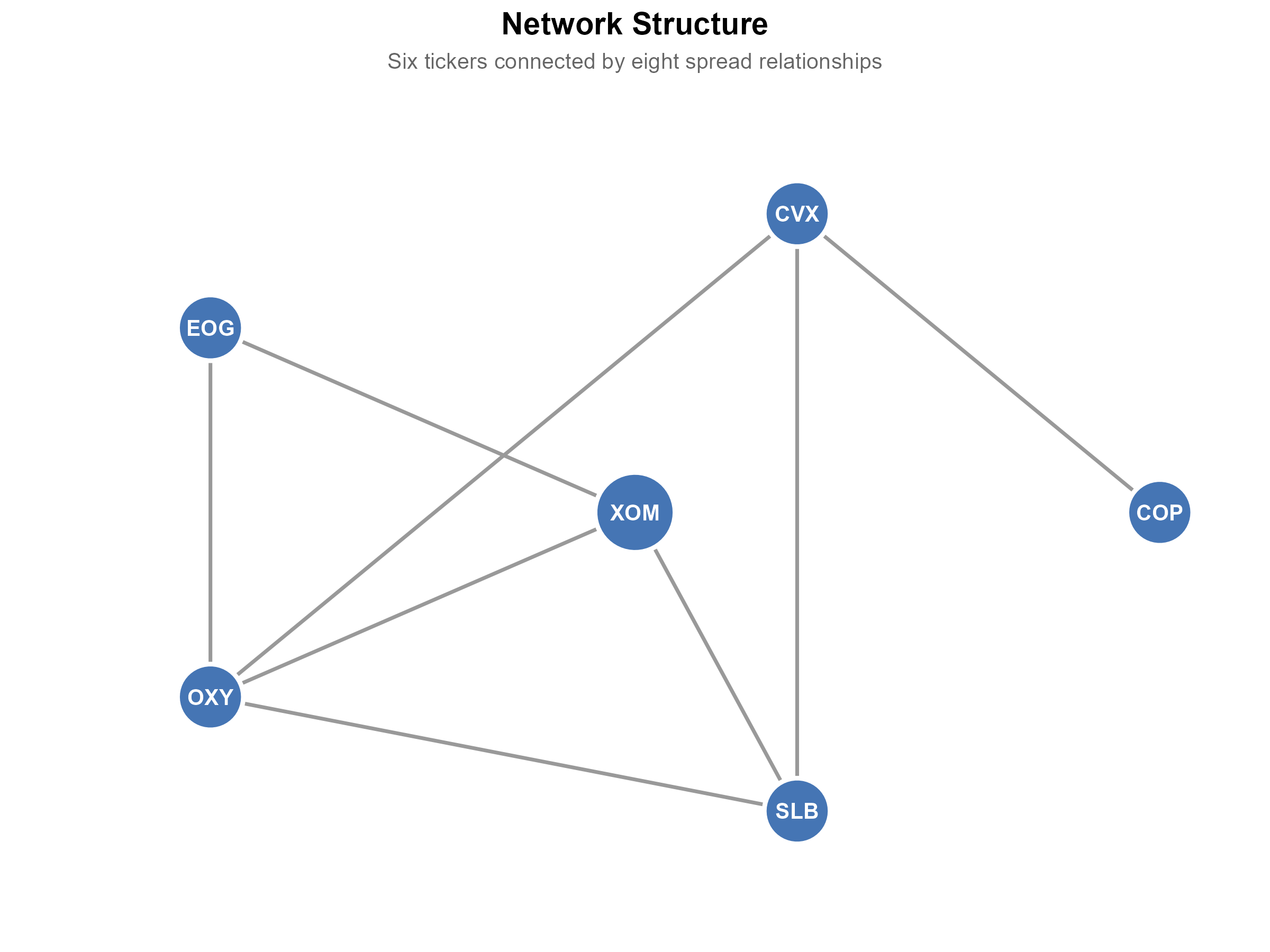
An edge between two ticker nodes indicates that those two tickers are connected in a spread.
We can visualise the state of the network at any point in time by incorporating the z-scores of each spread:
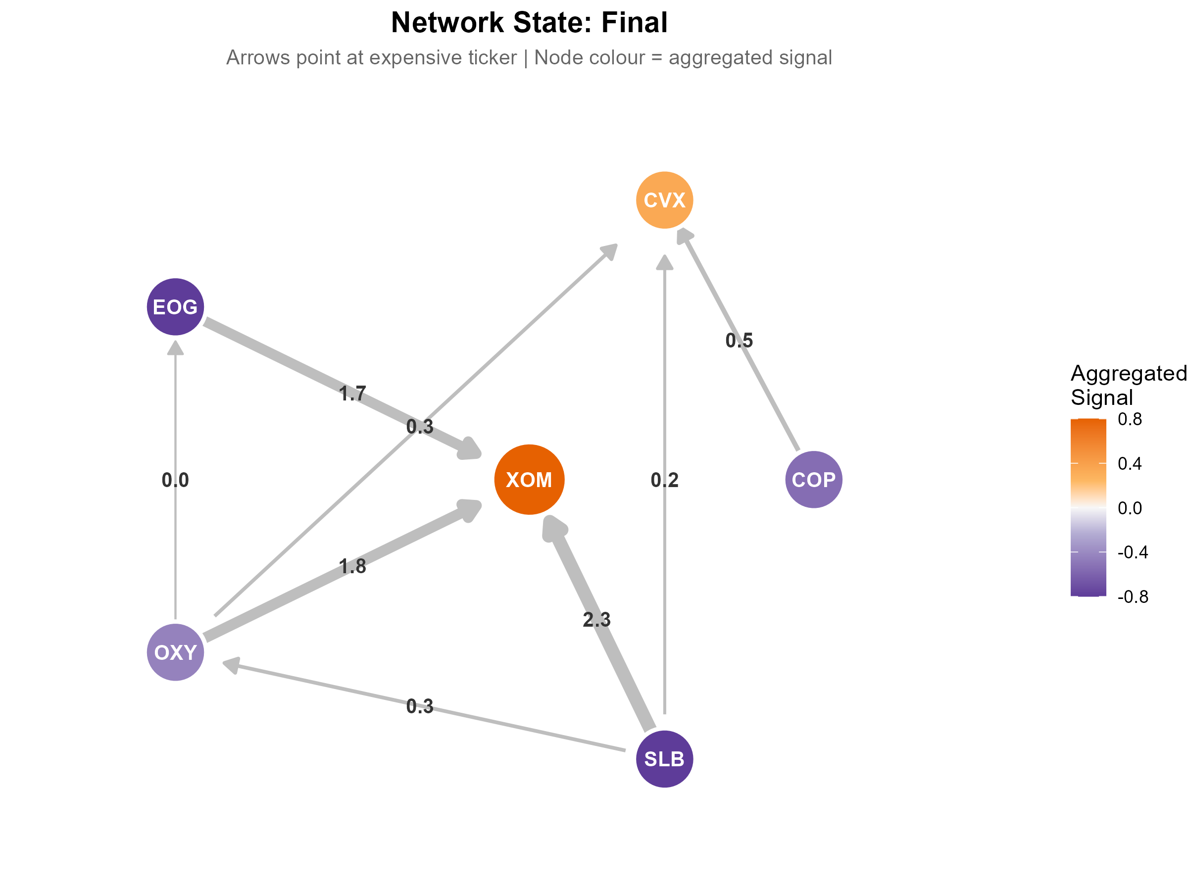
Arrows indicate the rich ticker in each pair (z-score positive)
The thickness of each connection represents the magnitude of the z-score
Thin shows a z-score close to zero
Thick shows a z-score that’s stretched
The colour of each ticker node represents that ticker’s aggregated z-score from all of its connections (orange = positive, purple = negative).
You can see how the state of the network evolves through time as the spreads diverge and converge:
The network gives you more information than any single spread can. When XOM is stretched against everyone, you have powerful collective evidence.
I call this Triangulated Stat Arb (not to be confused with triangular arbitrage, which is a different thing entirely.) We’ll get into exactly why that name makes sense in the next article.
For now, the key insight is this: instead of trading spreads, you trade the securities themselves. And instead of choosing between conviction and variance control, you get both. But you lose some simplicity.
Traditional pairs trading operates at the spread level. You see a divergent spread, you trade both legs, you wait for convergence.
The shift I’m describing operates at the ticker level. You use all those spreads as information about individual securities. Then you trade the securities directly.
The mechanics are straightforward. I call it “flattening” because you’re collapsing spread-level signals down to ticker-level signals.
Here’s how flattening works:
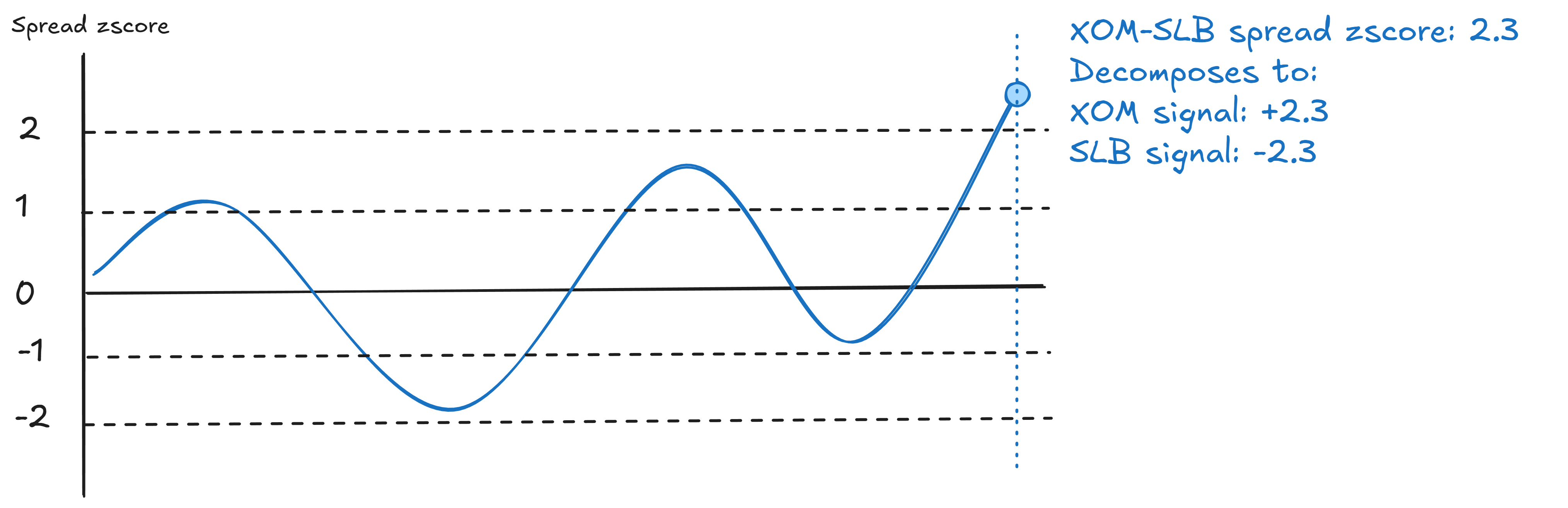
Take any spread signal at some point in time and decompose it into two ticker signals.
Say you’ve got the XOM-SLB spread with zscore +2.3. That means XOM is rich relative to SLB. So:
XOM gets +2.3 (appears expensive)
SLB gets -2.3 (appears cheap)
Same magnitude, opposite signs. One spread becomes two votes.
Do this for every spread in your universe at the current point in time. Now you’ve got a bunch of votes for each ticker. Some tickers appear in many spreads, some in few. Each spread casts a vote on both its legs.
Now aggregate. XOM appears in three spreads, all saying it’s rich. Average those signals. You get a strong positive aggregate. Strong positive means “this looks expensive.”
SLB appears in three spreads as well. One says it’s cheap (relative to XOM), the others say it’s roughly fair. The SLB signals disagree - weaker conviction. It’s probably not the mispriced leg in its one divergent spread.
This is the power of triangulated stat arb. Stuff that’s genuinely mispriced shows up as mispriced against multiple partners. Noise tends to wash out, while the signal gets reinforced.
With ticker-level signals, you build a long/short portfolio.
Tickers with strong negative signals (cheap against multiple partners) go in the long book. Tickers with strong positive signals (rich against multiple partners) go in the short book.
The key insight is that you’re not building a portfolio of “one mispriced leg plus one fair-value leg” repeated many times, as in a pair trade:
Instead, you’re building a portfolio of mispriced tickers. The longs are cheap. The shorts are rich.
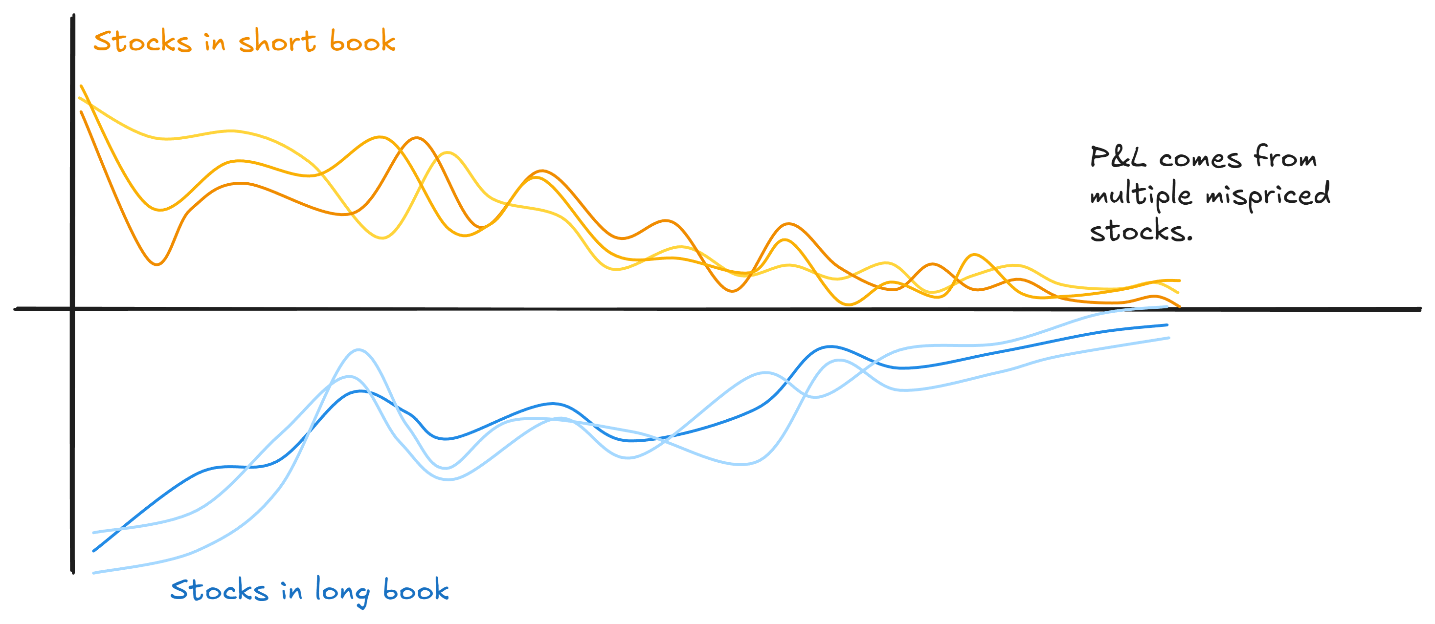
Both sides are working for you.
There are many ways you can construct a portfolio with this insight.
You’ll find that the effect tends to concentrate in the extremes, but there can be value in trading the broader distribution. It really depends on what else you’re doing and what you want to achieve.
If you want, you can size it so your net market exposure is roughly zero. This will give you similar variance reduction to pairs trading, but through portfolio construction rather than pair-by-pair hedging.
I’ve been letting the portfolio drift net long or net short, depending on the relative magnitude of the signals in the long and short books. This tends to juice returns at the expense of some higher variance.
There are many possible implementations, including weighting by the quality of the spreads the ticker-level signals come from, and accounting for how many times a ticker appears in the network (more votes lead to more conviction). More on these ideas later.
But essentially, this is the “have your cake and eat it too” part. You’re targeting the mispriced legs directly. But because you’re long a basket of cheap tickers and short a basket of rich tickers, you still get the low-variance benefits of a hedged approach.
This approach - triangulated stat arb - addresses the problems we identified in Part 3.
Capital efficiency. You’re deploying capital on legs that are actually mispriced. Not tying up half your position on fair-value hedges.
Signal utilisation. Remember the 100-pairs problem? Your selection pipeline identifies heaps of good pairs, but you could only trade 10 due to capital inefficiency. Now you’re aggregating information from your entire universe. More of your research actually gets used.
Lower transaction costs. You only pay for the legs that are actually mispriced.
Diversification. You’re holding positions in individual securities, not paired positions. More natural diversification (that you can dial up or down to fit your objectives).
Perhaps most exciting is that the portfolio approach can be incorporated into a broader multi-factor long/short portfolio - the aggregated pairs signals can be viewed as just another factor.
There’s something I haven’t fully addressed.
In our network of energy stock spreads, the case for XOM being mispriced was compelling. We had a lot of overlapping spreads all pointing in the same direction.
Often in practice, it won’t be that clean.
We might have sparser areas of the network with fewer connections. Stocks moving on noisy betas to their sector and the broader market can cloud things as well.
Figuring out which one moved helps, but it’s not definitive. What else can we use?
When do multiple spreads agreeing give you genuine conviction versus just coincidence? How do you measure the network’s agreement? How do you know when you’ve got a clearer signal versus noise?
That’s where triangulated stat arb really earns its name. The navigation metaphor provides a nice, simple mechanism for assessing the quality of an aggregated signal.
In the next article, I’ll show you how it works.
If you’re finding this useful, I share more practical thinking like this in my case study on how I went from corporate quant to independent trader. Grab it here.
I’m loving this series! Did you use a rolling hedge ratio inside your z-score graphs? I’m curious how the spread was constructed.